Neural Ordinary Differential Equations: Continuous Depth

Introduction

Neural Ordinary Differential Equations allow you to define neural networks with continuous depth. Apart from theoretically being interesting, using such models you can define continuous time series models for forecasting or interpolation or continuous normalizing flows.

In this blog post first, we will begin with a review on numerical methods for solving initial value problems as an introduction to the idea of Neural ODE. Then we will see how to implement such networks in PyTorch using TorchDiffEq.

Initial Value Problems and Numerical Solutions

As you may already know an initial value problem is defined as follows.
Given a function $f(t, y)$ and an initial value $y_0$, find a function $y$ which satisfies the differential equation:

\[\frac{dy}{dt} = f(t, y)\]

And further satisfying the initial condiotion $y(0) = y_0$.
The difficulty of solving such initial value problems depends on the RHS of the above equation $f(t, y)$. In most cases, there is no analytical method to solve it and it can only be solved if $f(t, y)$ has specific forms. However, there are some numerical methods for approximating the solution $y$.
Perhaps the simplest numerical approach to solve an ODE is to use the Euler method. The idea is simple. a differential equation describes changes in the value of a function. So starting with the initial value $y_0$ we can construct a solution step-by-step as in each step $t_n$ the equation tells us how to change the current value $y_n$ to compute the next value $y_{n+1}$. Using Taylor expansion we can derive the following update:

\[y_{n+1} = y_n + mf(t_n, y_n)\]

Where $m$ is the step size. Smaller step sizes give a more accurate approximation. As an example consider the initial value problem:

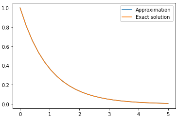
\[\frac{dy}{dt} = -y\]

with the initial condition $y(0) = 1$. In this case the exact solution is $y = e^{-t}$. But Let’s try to approximate it using the Euler method over the interval $[0,5]$:

def f(t, y):
  return -y

step = 0.2
steps = np.linspace(0, 5, num=int(5/step))
y_app = np.zeros_like(steps)
# initial condition
y_app[0] = 1.0

for n in range(len(steps)-1):
  y_app[n+1] = y_app[n] + step*f(steps[n], y_app[n])

Plotting the approximated solution versus the exact values of $y$ shows even a simple method like Euler can be useful:
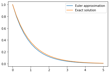
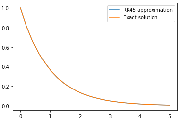
Euler approximation vs the exact solution
People use more accurate techniques to integrate ODEs like Runge-Kutta. Some methods even use adaptive step sizes. You can use scipy package to solve initial value problems. For example to solve the same problem we can use a variant of the Runge-Kutta methods:

from scipy.integrate import solve_ivp
solution = solve_ivp(f, (0, 5.0), y0=[1.0], method='RK45', t_eval=steps)

And the result shows a more accurate approximation:
Euler approximation vs the exact solution

Great! But how do initial value problems relate to continuous depth?

Neural ODE

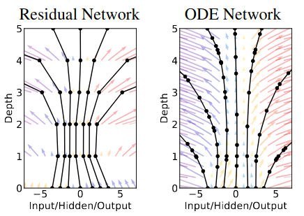
Now consider a simple recurrent neural network. In such networks, we apply a sequence of transformations on a hidden state. For the sake of simplicity suppose in each layer we apply a simple nonlinear transformation $f$ parameterized by a vector of parameters $\theta$ which might be time-dependent so let’s call it $\theta_t$ where $t$ denotes the time step. So we begin with an initial hidden state $h_0$ and update it according to the following iteration for a number of steps $T$:

\[h_{t+1} = h_t + f(h_t, \theta_t)\]

Now If you look closely, This update is very similar to what we did in the Euler method to solve an initial value problem. It seems the RNN is trying to solve an initial value problem, so by making the step size smaller and smaller and increasing the number of layers in the limit to infinity we have:

\[\frac{d\mathbf{h(t)}}{dt} = f(\mathbf{h}(t), t, \theta)\]

Here $f$ is a neural network parameterized by $\theta$. Now we can define $h(T)$ as the output of this network which is called Neural Ordinary Differential Equation a parameterized differential equation.

How to train a Neural ODE?

After defining Neural ODE the main question is How to train it? To find a proper parameter vector $\theta$ which minimizes a loss function $L$, we need to compute the gradient of the loss function. Obviously, we have to compute $h(T)$ as we have defined it as the output of the network. Since this is a differential equation we can compute $h(T)$ by solving as initial value problem using a numerical solver like the Euler method. Don’t forget we have to compute the gradient of some loss functions which depends on $h(T)$. But can we differentiate through an ODE solver? Recall what we did in the Euler method once again, anything we did was differentiable so it seems differentiating through an ODE solver is straightforward and can be done using automatic differentiation systems like Autograd in PyTorch. However, a great advantages of Neural ODE is that we can perform this gradient computation much more efficiently.

Adjoint Sensitivity Method

One of the problems associated with deep neural networks is the cost of gradient computation which increases as we add more layers to the model, Interestingly it turns out in the case of Neural ODE we can do this with constant memory using a method called Adjoint Sensitivity. Adjoint methods are a family of gradient computation methods applicable to certain problems.

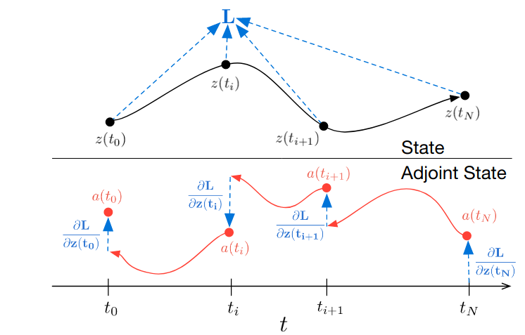
As we have seen in the Euler method, the solver approximates the solution step-by-step. Let’s use $z(t)$ to denote the output(state) of the solver at time step $t$. Instead of directly computing the gradient of the loss function $L$ we may define:

\[\mathbf{a}(t) = \frac{\partial L}{\partial \mathbf{z}(t)}\]

Here $\mathbf{a}(t)$ is called the adjoint. adjoint is obviously a function of time and as its definition suggests is the sensitivity of loss to a change in the value of state $\mathbf{z}(t)$. The dynamics of adjoint is described by a differential equation:

\[\frac{d\mathbf{a}(t)}{dt} = -\mathbf{a}(t)^{T}\frac{\partial f(\mathbf{z}(t), t, \theta)}{\partial \mathbf{z}}\]

Using both values of $\mathbf{a}(t)$ and $\mathbf{z}(t)$ the gradient of $L$ can be computed as follows using an ODE solver:

\[\frac{dL}{d\theta} = - \int^{t_0}_{t_1}\mathbf{a}(t)^{T}\frac{\partial f(\mathbf{z}(t), t, \theta)}{\partial \theta} dt\]

Where $[t_0, t_1]$ is the interval of time steps over which we approximate the ODE solution.

Solving Initial Value Problems using torchdiffeq

The paper of Neural ODE comes with a python package called torchdiffeq to make gradient computation using the adjoint method easier. Install the package using pip:

pip install torchdiffeq

Let’s see how to use it to solve an initial value problem. consider the same problem discussed earlier. Just like before you need to define $f(t, y)$ but now we define it as a PyTorch module:

import torch
import torch.nn as nn

class F(nn.Module):
  def forward(self, t, y):
    return -y

Now using torchdiffeq we can solve it as we used scipy but this time using the adjoint method:

from torchdiffeq import odeint_adjoint as odeint
# creating f(t,y)
func = F()
# the timesteps we need the value of y
t = torch.linspace(0, 5.0, 25)
# initial condition y(0)
y0 = torch.tensor([[1.0]])
# solving the IVP
y_app = odeint(func, y0, t)

And the result is again what we expected:
The Solution of torchdiffeq
Although everything seems just like scipy but now we are free to define $f(t,y)$ using a neural network. for example:

class F(nn.Module):
  def __init__(self):
    super().__init__()

    self.net = nn.Sequential(nn.Linear(1, 8),
                             nn.Tanh(),
                             nn.Linear(8, 1))
  
  def forward(self, t, y):
    return self.net(y) * t

In this case, solving the problem is the same as before:

func = F()
t = torch.linspace(0, 5.0, 5)
y0 = torch.tensor([[-1.2]])
y_app = odeint(func, y0, t)

But after checking the solution tensor we can see the computation graph needed to compute the gradient is saved:

tensor([[[-1.2000]],
        [[-1.5032]],
        [[-2.3417]],
        [[-3.5586]],
        [[-5.1382]]], grad_fn=<OdeintAdjointMethodBackward>)

The gradient can be computed by simply calling backward on the output of some loss function. At this time we are ready to implement a continuous time series model using Neural ODE.

Example : A Continuous Time Series Autoencoder

Problem Definition

In this section we are going to see how to use Neural ODE to design a continuous time series autoencoder model. Such a model can be useful for time series interpolation, representation learning, or forcasting. Let’s create a synthetic time series with irregular observations. TimeSynth is a lightweight python library for generating different types of time series data. First, install it using pip:

pip install git+https://github.com/TimeSynth/TimeSynth.git

Using TimeSynth you can synthesize a time series using various types of signal and noise processes. For example, here we use a Gaussian Process with a Matern kernel as a signal and an additive Gaussian noise to create the time series.

import timesynth as ts

# Initializing a Gaussian Process signal with a Matern kernel
signal_process = ts.signals.GaussianProcess(kernel='Matern')
# Initializing Gaussian noise
white_noise = ts.noise.GaussianNoise(std=0.1)
# Initializing TimeSeries class with the signal and noise objects
timeseries = ts.TimeSeries(signal_process, noise_generator=white_noise)

In the above code timeseries is a generative process and we can sample from it. To do so we need to specify a set of time points for sampling. we use irregular time steps for this.

# time steps to sample the time series
samples = np.sort(np.random.uniform(0, 5, 60))
# sampling the time series
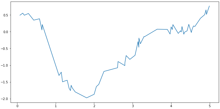
series, signal, noise = timeseries.sample(samples)

Plotting the generated series and you will see something like this:

plt.plot(samples, series)

Regular time series
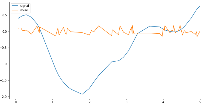
We can also plot the signal and noise separately:

plt.plot(samples, signal, label='signal')
plt.plot(samples, noise, label='noise')
plt.legend()

Regular time series with separated signal and noise
So far we have a time series with irregular observations. Using a continuous time autoencoder we can interpolate arbitrary time points and use them for forecasting. There are many other applications for a continuous autoencoder like denoising, forecasting, …

Model Specification

The overall architecture of the autoencoder has been shown in the figure below:
An encoder network will encode the series to produce a latent vector $z_0$. This latent vector can be used as the initial condition of the Neural ODE. By solving the Neural ODE we can obtain the latent representation of each time steps $z_{t_0}, z_{t_1}, …, z_{t_n}$. You may ask why the ODE should generate the latent points? The reason is in this case we will be able to sample the encoded series in arbitrary time points.
Autoencoder

Neural ODE is responsible to model the dynamics of the latent space. Encoders usually describe the latent space itself. But in this model we first describe the dynamics of latent space and then generate the latent space by solving the Neural ODE. The Neural ODE is as follows:

class Encoder_ODE(nn.Module):
  def __init__(self, latent_dim):
    super().__init__()

    self.latent_dim = latent_dim
    self.net = nn.Sequential(nn.Linear(self.latent_dim+1, self.latent_dim),
                             nn.CELU(),
                             nn.Linear(self.latent_dim, self.latent_dim))
   
    self.omega = nn.Parameter(torch.rand((1,)))
    
  def forward(self, t, y):
    # handling seasonality
    time = torch.sin(self.omega*t.view(1, 1))
    combined = torch.cat([time, y], dim=1)
    return self.net(combined)

For decoding the latent values we can define a simple MLP which acts on each latent time point $z_i$ separately. This way it is easier to generate the series in arbitrary points after training the Autoencoder.

class AE(nn.Module):
  def __init__(self, latent_dim):
    super().__init__()

    self.latent_dim = latent_dim
    self.ode = Encoder_ODE(self.latent_dim)
    self.lstm_encoder = nn.LSTM(1, self.latent_dim, batch_first=True)
    self.fc_decoder = nn.Sequential(nn.Linear(self.latent_dim, self.latent_dim),
                                    nn.Tanh(),
                                    nn.Linear(self.latent_dim, 1))
  
  def forward(self, t, y):
    # zero initialized hidden vector
    (h0, c0) = (torch.zeros(1, 1, self.latent_dim),
                torch.zeros(1, 1, self.latent_dim))
    # encoding the time series
    _, (h, c) = self.lstm_encoder(y.view(1, -1, 1), (h0, c0))

    # using the last hidden value as the initial condition for solving ODE 
    z0 = h[0]
    # generating the latent points by solving ODE
    z = odeint(self.ode, z0, t_train).squeeze()
    y_decoded = self.fc_decoder(z)
    return y_decoded

Before training, We need to change the training data to PyTorch tensors.

t_train = torch.from_numpy(samples).float()
y_train = torch.from_numpy(series).float()

We can now instantiate the autoencoder. Since we want to use this models for interpolating only one time seires, I use a small latent dimension latent_dim = 3.

import torch.optim as optim
model = AE(latent_dim=3)
optimizer = optim.Adam(model.parameters(), lr=0.002)
criterion = nn.MSELoss()

Now the model is ready for training

loss_track = []
epochs = 300
for epoch in range(epochs):
  # set the accumulated gradient in tensors to zero
  optimizer.zero_grad()
  y_decoded = model(t_train, y_train)
  # computing the reconstruction loss
  train_loss = criterion(y_decoded.squeeze(), y_train)
  # computing the gradient using backprop
  train_loss.backward()
  # updating the parameters using the optimizer
  optimizer.step()
  loss_track.append(train_loss.item())

To train Neural ODE choosing a proper learning rate for optimizer is important. Loss per epochs
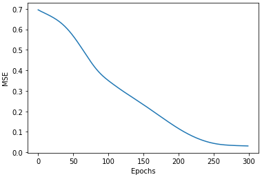
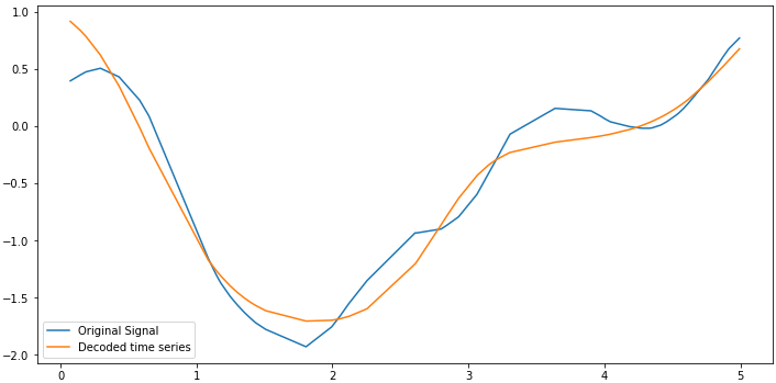
Finally we can plot the decoded series vs the original signal which had been used to define the time series processs. Now you can use the model to sample arbitrary time points from time series. Decoded Series vs Original Signal

References

Neural Ordinary Differential Equations, Ricky T. Q. Chen, Yulia Rubanova, Jesse Bettencourt, David Duvenaud, arXiv:1806.07366v5 [cs.LG]
Slides from MIT Course on Multidisciplinary System Design Optimization, lecture 9 Gradient Calculation and Sensitivity Analysis, Olivier de Weck, Karen Willcox