Wasserstein Auto-Encoders | Probabilistic OCR

Probabilistic Optical Character Recognition

Suppose someone asks you to detect the letter behind the rectangle in the following image:

Not sure. It may be either a “C” letter or “O” or “G”.In fact the answer to the question is not a letter but a probability distribution over letters with a mass function like this:

\[p("O") = 0.44, p("C") = 0.33, p("G") = 0.10, ...\]

Given the information we have, that’s the best answer we can give. Likewise, it’s not clear whether the word in this image is “clear” or “clean” or “cleat”:

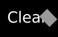
Again the answer is not a word but a distribution over words. What I’m trying to say is that OCR is inherently a probabilistic task due to the uncertainty that lies in the answer. In this article, I’ve explained how to construct a probabilistic OCR model and finally the implementation of the model in PyTorch.

Defining A Probability Distribution Over Words

There are many ways to define a probability distribution over sequence data like text. For example, one can use Markov models. However, in this article, I wanna explore another approach that circumvents the difficulty of defining a distribution over a sequence of characters by learning a distributed representation of words. Since it’s easy to construct a probabilistic model for continuous variables we can try to learn a continuous representation of data. Yeah, some sort of embedding but different from usual word embeddings methods that are based on words’ semantics.

Repesentation Learning using Wasserstein Auto-Encoder

Auto-Encoder is a famous neural network architecture that is well known for the ability to learn a very nice lower-dimensional representation of data. There are various types of Auto-Encoders, The model we are going to use is a rather new one called Wasserstein Auto-Encoder (WAE). To understand WAE we will briefly review the standard Auto-Encoders then Variational Auto-Encoders and finally Wasserstein Auto-Encoders.

Standard Auto-Encoder

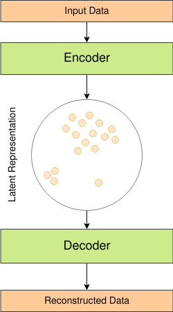
A Standard Auto-Encoder (AE) contains two blocks namely Encoder and Decoder. The encoder is a neural network that maps the original data into the lower dimensional space and the Decoder as its name suggests tries to decode that lower-dimensional representation.

Usually, people design Encoder and Decoder to be symmetric. In the case of words and more generally sequence data, Among the popular choices are RNNs, CNNs, Transformers, or just simple MLPs. Whatever the architecture, To reconstruct the data, the learned representation has to contain the most important information. AE tries to minimize the error of data reconstruction $c$ a function which can be a distance like MSE.

\[\mathrm{Loss} = \sum^{n}_{i=0} c(x_i, \bar{x}_i)\]

However, The problem is all of the representations are not necessarily feasible. So some variants try to impose a prior belief over the representation in order to have a representation with specific properties like being disentangled. Perhaps the most popular model of this kind is Variational Auto-Encoder.

Variational Auto-Encoder

Variational Auto-Encoder (VAE) aims to not only minimize the reconstruction loss but also try to make the distribution of learned representation similar to a prior distribution. The prior can be simply a Gaussian distribution or a mixture model or even a complicated density like a Normalizing Flow. Hence the loss of VAE can be written as follows:

\[\mathrm{Loss} = \sum^{n}_{i=0} c(x_i, \bar{x}_i) + D(p(Z), q(Z))\]

such that $Z$ is the learned representation (latent), $p$ is the distribution of latent representation and $q$ is the target prior distribution. Finally, $D$ must measure a distance between $p$ and $q$. The original VAE paper uses Kullback–Leibler divergence as distance:

\[\mathrm{Loss} = \sum^{n}_{i=0} c(x_i, \bar{x}_i) + D_{\mathrm{KL}}(p(Z)||q(Z))\]

KL divergence is a member of a more general family called f-divergence.

Wasserstein AutoEncoder

Another idea for making distributions $p$ and $q$ similar to each other is minimizing maximum mean discrepancy (MMD) which is defined as follows:

\[\mathrm{MMD}(p(Z), q(Z)) = \frac{1}{n(n-1)}\sum_{l\neq j}k(z_l, z_j) + \frac{1}{n(n-1)}\sum_{l\neq j}k(\tilde{z}_l, \tilde{z}_j) - \frac{2}{n^2}\sum_{l, j}k(z_l, \tilde{z}_j)\]

Where in the above formula, $k$ is a positive-definite kernel, $z$ denotes the samples from prior $q$, and $\tilde{z}$ will be sampled from learned representation. MMD works well especially on high dimensional Gaussian densities. So when using a Gaussian distribution as prior, MMD can be a good choice. This formulation is a special type of Wasserstein Auto-Encoder. Our final loss function is as follows:

\[\mathrm{Loss} = \frac{1}{n}\sum^{n}_{i=0} c(x_i, \bar{x}_i) + \lambda D_{\mathrm{MMD}}(p(Z), q(Z))\]

Where $\lambda$ controls the effect of MMD term that acts as a regularizer.

PyTorch Implementation

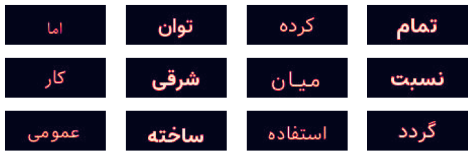
Implementation of WAE using PyTorch is easy but let us first explore the data we are going to use. We want to construct an OCR model on the Shotor dataset. Shotor is a free synthetic word-level OCR dataset generated for the Persian language. OCR for Persian is difficult since, in Persian, characters are connected to each other. The dataset contains 2M images with the size of $40\times 100$ and corresponding text in addition to other information like the fonts used to generate the image. Here is a sample batch of images in the dataset.

Importing Modules

import os
import pandas as pd
import numpy as np

import matplotlib.pyplot as plt
import seaborn as sns
sns.set()
sns.set_style('dark')


import torch
import torch.nn as nn
import torch.optim as optim
import torch.distributions as td
from torch.utils.data import Dataset, DataLoader
from torchvision import transforms


import cv2 as cv

Data Preparation

First we need to define all Persian alphabets and map each one to an index.

pchars = "آ ا ب پ ت ث ج چ ح خ د ذ ر ز ژ س ش ص ض ط ظ ع غ ف ق ک گ ل م ن و ه ی ئ"
pchars =  ['E', ' '] + pchars.split(' ')
letter_to_index = {}
for i in range(len(pchars)):
  letter_to_index[pchars[i]] = i
index_to_letter = {v:k for k,v in letter_to_index.items()}

The images in the datasets are $40 \times 100$ but we will resize them to $25 \times 50$

# input images width
img_width = 50
# input images height
img_height = 25

Now we set a maximum word length. To make sure all of the words have the samle length we have to pad them later. Also we use mini batches with size of $16$.

# maximum length of each word
word_max_len = 11
# device for tensors
device = 'cpu'
batch_size = 16
num_chars = len(pchars)

Next we should read the csv file containing images’ path and labels.

dataset_path = './images/'
csv_words_path = './shotor.csv'
# read the words file
words_csv = pd.read_csv(csv_words_path)

To make dataset usage easier we can use PyTorch Dataset.

class PersianOCR(Dataset):
    def __init__(self, words_csv, root_dir, transform=None):
        self.root_dir = root_dir
        self.transform = transform
        self.csv = words_csv.reset_index(drop=True)

    def __len__(self):
        return self.csv.shape[0]

    def __getitem__(self, idx):
        if torch.is_tensor(idx):
            idx = idx.tolist()
        img_name = os.path.join(self.root_dir,
                                self.csv.iloc[idx, 0])
        word = self.csv.iloc[idx, 1]
        image = cv.imread(img_name, cv.IMREAD_GRAYSCALE)
        
        item = {'image': image, 'word': word}

        if self.transform:
            item = self.transform(item)

        return item

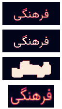
In a real-world OCR application, we first need to detect a rectangle containing the word using object detection. However, in this simple dataset, we can do this by finding contours. But before that, we use dilation to connect all pixels of a word. Here is an example of this procedure:

We define the above procedure as a PyTorch transformation using OpenCV:

class CropWord():
  def __call__(self, sample):
      image, word = sample['image'], sample['word']
      
      ret, thresh = cv.threshold(image, 0, 255, cv.THRESH_OTSU | cv.THRESH_BINARY)
      rect_kernel = cv.getStructuringElement(cv.MORPH_RECT, (3, 3))
      dilated = cv.dilate(thresh, rect_kernel, iterations = 4)
      cnt, h = cv.findContours(dilated, 1, 2)
      if(len(cnt) > 0):
        x,y,w,h = cv.boundingRect(cnt[0])
        extracted_word = cv.resize(image[y:y+h, x:x+w], (img_width, img_height))
      else:
        extracted_word = cv.resize(image, (img_width, img_height))
      
      return {'image': extracted_word,
              'word': word}

For feeding images and labels to PyTorch model we must convert numpy arrays to PyTorch Tensors:

class ToTensor(object):
  """Convert ndarrays in sample to Tensors."""
  def __call__(self, sample):
      image, word = sample['image'], sample['word']
      image = image.reshape(-1, img_height, img_width)/255.0
      if (len(word) > word_max_len):
        word = word[:word_max_len]
      word = word + 'E' * (word_max_len - len(word))
      original_word = [letter_to_index[c] for c in word]
      return {'image': torch.from_numpy(image).float().to(device),
              'word_tensor' : torch.LongTensor(original_word).to(device),
              'word': sample['word']}

Dataset contains 2M images but we only use 200000 records for training.Now we can define a dataloder to create mini batchs automatically.

df_shuffle = words_csv.sample(frac=1.0, random_state=0)
train_df = df_shuffle[:200000]

train_dataset = PersianOCR(train_df, dataset_path,
                           transform=transforms.Compose([CropWord(),
                                                         ToTensor()]))

train_dataloader = DataLoader(train_dataset, batch_size=batch_size, shuffle=False)

Model Definition

Let’s begin with Wasserstein Auto-Encoder.

WAE

The diagram of the WAE that we going to imlement is depicted in the below figure:

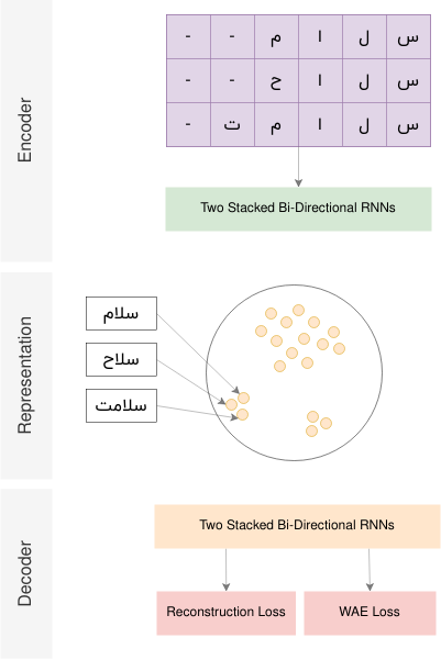
For the encoder block we use two bi-directional RNNs:

class WordEncoder(nn.Module):
  def __init__(self, latent_size, char_emb_size):
    super().__init__()

    self.latent_size = latent_size
    self.char_emb_size = char_emb_size

    self.char_emb = nn.Embedding(num_chars, char_emb_size)

    self.rnn_enc = nn.RNN(char_emb_size, latent_size, bidirectional=True,
                          num_layers=2)
    

  def forward(self, word):
    bsize = word.size(0)
    word = self.char_emb(word)
    word = word.permute(1, 0, 2)
    h0 = torch.zeros(4, bsize, self.latent_size).to(device)
    out, h0 = self.rnn_enc(word, h0)
    h0 = h0.permute(1, 0, 2)
    latent = h0.mean(dim=1)
    return latent

Also for the Decoder block we use the sample architecture as Encoder but in reverse order:

class WordDecoder(nn.Module):
  def __init__(self, latent_size, rnn_hidden):
    super().__init__()

    self.latent_size = latent_size
    self.rnn_hidden = rnn_hidden

    
    
    self.rnn_dec = nn.RNN(latent_size, num_chars, bidirectional=True,
                          num_layers=2)
    
    self.unflatten = nn.Unflatten(2, (2, -1))

  def forward(self, latent):
    bsize = latent.size(0)
    latent = latent.unsqueeze(0).expand(word_max_len, bsize, self.latent_size)
    h = torch.zeros((4, bsize, self.rnn_hidden)).to(device)
    out, h = self.rnn_dec(latent, h)
    word = out.permute(1, 0, 2)
    word = self.unflatten(word)
    word = word.mean(2)
    return word

As I said before in the definition of maximum mean discrepancy, we need a positive definiate kernel $k$. we can use squared exponential kernel:

\[k(z_i,z_j) = e^{-||z_i-z_j||^2_2}\]

To implement this kernel efficiently I used PyTorch cdist that can compute distances of a batch in a GPU compatible way.

Since the WAE is actually classifying each decoded character, we can use Cross-Entropy as the reconstruction loss function. Finally, we use a Gaussian prior to learning a disentangled representation.

class WAE(nn.Module):
  def __init__(self, latent_size):
    super().__init__()

    self.latent_size = latent_size
    
    self.encoder = WordEncoder(latent_size, 16)
    self.decoder = WordDecoder(latent_size, 36)

    self.prior = torch.distributions.Normal(torch.tensor(0.0).to(device),
                                            torch.tensor(2.0).to(device))
    
    self.lam = 1

  def kernel(self, z1, z2):
    return torch.exp(-torch.cdist(z1, z2))

  def forward(self, word):
    z = self.encoder(word)
    rec_word = self.decoder(z)
    return rec_word, z
  

  def mmd_loss(self, word):
    rec_word, z_bar = self.forward(word)
    z = self.prior.sample(z_bar.shape)
    
    n = z.size(0)
    k_z_z = self.kernel(z,z)
    k_zb_zb = self.kernel(z_bar, z_bar)
    k_z_zb = self.kernel(z, z_bar)

    
    true_chars = word.flatten()
    decoded_chars = torch.cat(list(rec_word), dim=0)
    loss = nn.functional.cross_entropy(decoded_chars, true_chars)

    loss = loss + (self.lam/(n*(n-1)))*(k_z_z.sum() - torch.diagonal(k_z_z).sum())
    loss = loss + (self.lam/(n*(n-1)))*(k_zb_zb.sum() - torch.diagonal(k_zb_zb).sum())
    loss = loss - (2*self.lam/(n))*k_z_zb.mean()
    return loss, rec_word, z_bar

A Probabilistic OCR Model

Remember the final goal was to construct a probabilistic model for OCR. The output of this model can be a distribution over the representation learned by WAE. Since the representation is continuous we can use a multivariate Normal density. To reduce the number of parameters I used a diagonal covariance matrix. Now the OCR model takes the images as input and then gives the parameters of the Normal distribution as output namely the mean and covariance matrix. To train this model we can maximize the likelihood of this Gaussian density or equivalently minimize the negative log-likelihood.

class OCR(nn.Module):
  def __init__(self, latent_size):
    super().__init__()

    self.latent_size = latent_size

    self.gru = nn.GRU(75, latent_size, bidirectional=True)
    
    self.mu = nn.Linear(latent_size, latent_size)
    self.log_sigma = nn.Linear(latent_size, latent_size)

  def forward(self, img):
    bsize = img.size(0)
    img = img.squeeze(dim=1).unfold(dimension=2, size=3, step=1).permute(2, 0, 1, 3)
    img = img.flatten(2)
    h0 = torch.zeros(2, bsize, self.latent_size).to(device)
    _, h = self.gru(img, h0)
    h = h.permute(1, 0, 2)
    h = h.mean(dim=1)
    mu = self.mu(h)
    log_sigma = self.log_sigma(h)
    sigma = torch.exp(log_sigma)   
    cov_matrix = torch.diag_embed(sigma)

    density = td.MultivariateNormal(mu, cov_matrix)
    return density

Now we create the models and set the dimension of latent space to 64.

torch.manual_seed(0)
ocr = OCR(64).to(device)
wae = WAE(64).to(device)

To get a prediction we can decode the mean of output density using the decoder. It’s better to define a helper function for training:

def train(epochs):
  for epoch in range(epochs):
    for i_batch, batch in enumerate(train_dataloader):

      true_word = batch['word_tensor']
      image = batch['image']

      wae_optimizer.zero_grad()
      mmd_loss, decoded_word, latent_target = wae.mmd_loss(true_word)
      mmd_loss.backward()
      wae_optimizer.step()

      ocr_optimizer.zero_grad()
      density = ocr(image)
      nll = -density.log_prob(latent_target.detach()).mean()
      nll.backward()
      ocr_optimizer.step()

Finally, we train both WAE and OCR models simultaneously for $4$ epochs. Note after each epoch we divide the learning rate by $5$

from madgrad import MADGRAD
for i in range(4):
  ocr_optimizer = MADGRAD(ocr.parameters(), lr=0.001/5**i)
  wae_optimizer = MADGRAD(wae.parameters(), lr=0.001/5**i)
  train(1)

I used MADGRAD optimizer. It’s not included yet in PyTorch optim so you need to install it:

pip install madgrad

After training you can define some helper functions to decode the output like these:

def tensor_to_word(tensor):
  indices = tensor.argmax(1)
  word = []
  for index in indices:
    word.append(index_to_letter[index.item()])
  word = ''.join(word)
  word = word.replace('E', '')
  return word

def mean_prediction(image):
  words = []
  with torch.no_grad():
    mean_latent = ocr(image).mean
    decoded = wae.decoder(mean_latent)
    for i in range(image.size(0)):
      words.append(tensor_to_word(decoded[i]))
  return words

Here I’ve created a visualization of learned representation and OCR output during training. In this video colors denote length of words.

References

• Wasserstein Auto-Encoders, Ilya Tolstikhin, Olivier Bousquet, Sylvain Gelly, Bernhard Schoelkopf, arXiv:1711.01558 [stat.ML]
• Auto-Encoding Variational Bayes, Diederik P Kingma, Max Welling, arXiv:1312.6114 [stat.ML]

Please cite my blog post if you want to use this project. Thanks!