Bayesian Stochastic Geometry

I was exploring the applications of Gaussian Processes in Stochastic Geometry, specifically for defining random curves. I thought it might be interesting to use a non-parametric model for representing curves and in general for geometric objects. So in this post, first we’ll see how to use Gaussian Processes for defining a distribution over 2D curves. Then we try to perform Bayesian inference for a shape completion task and finally an application for probabilistic motion planning.

Stochastic Geometric Objects

Uncertainty can arise in any kind of data and geometric objects are no exception. This is exactly the topic of Stochastic Geometry in which we study random geometric objects and the associated stochastic processes. This is really fun, for example, suppose you have a set of random lines, what would be the expected number of intersections? As you can guess there are a lot of questions concerning such random processes. In this post, I want to explore two problems namely shape completion and motion planning from a Bayesian perspective. Suppose we have a few data points from an unknown shape like this:

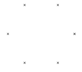
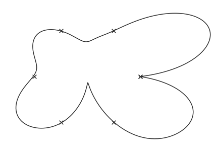
The question is can we find the complete shape given these 6 points? Of course, these points can belong to any geometric object. for example, it might be a circle, a polygon, or maybe some irregular shape like this:

From a Bayesian point of view, each shape passing through these points is a Hypothesis. Our desire is to define a distribution over possible hypotheses. To do this in a non-parametric way, we are going to use Gaussian Processes.

Gaussian Processes

Gaussian Process is a famous stochastic process used as a non-parametric Bayesian model to define a distribution over functions. The properties of sampled functions can be determined by a mean and a covariance function. Commonly people use a zero mean for priors and the interesting part is choosing the covariance function or the kernel. Different kernels lead to different families of functions and designing kernels for Gaussian Processes is a hot research topic. we will see how the choice of kernel affects the enerated curves. I don’t discuss GP definition and inference methods here so check out [1] for the definition, inference, and applications of GP in machine learning. In this post, I’ll denote GP by $\mathcal{Gp}(\mathbf{\mu}, \mathbf{\Sigma})$ where $\mathbf{\mu}$ and $\mathbf{\Sigma}$ are the mean and the covariance function respectively.

A simple prior over curves

To define a prior over 2D curves, one way is to parameterize the curve and use a Gaussian Process for each component. However, for the sake of simplicity for now, let’s switch to the polar coordinates so we can use a single GP. This is not equivalent to the former method but since we are interested in shape completion, the result will be satisfying.

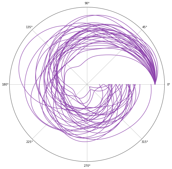
\[\theta \in [0,2\pi]\] \[r(\theta) \sim \mathcal{Gp}(\mathbf{\mu}, \mathbf{\Sigma})\]

Let’s choose a Rational-Quadratic kernel defined as follows:

\[k(x_i, x_j) = (1 + \frac{d(x_i, x_j)^2}{2\alpha l^2})\]

Here are some curve sampled from this prior.

Samples from the prior defined by a Rational-Quadratic Kernel

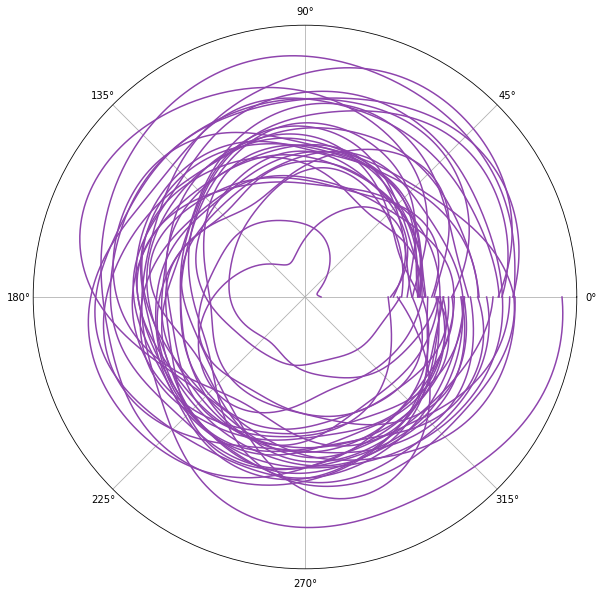
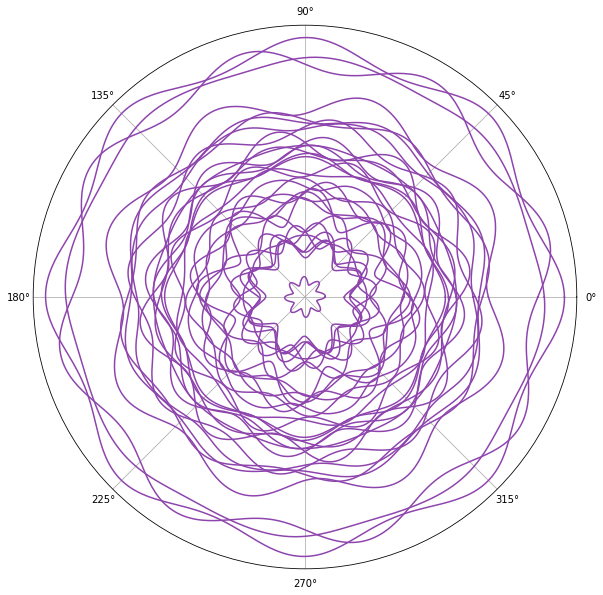
As you can see in the above plot, The curves haven’t formed closed shapes. Of course, we can define some constraints to enforce this but there is a simpler way. In Gaussian Process and more generally in any Bayesian method, prior is a way for injecting domain knowledge. Since our goal is to model shapes using these curves, we can enforce this constraint by choosing a more suitable prior. For example, we can use Exponential-Sine which is a periodic kernel:

\[k(x_i,x_j) = \exp{(-\frac{2\sin^2(\pi d(x_i,x_j)/p)}{l^2})}\]

By choosing a suitable period length for example $p=\frac{\pi}{4}$ we make sure $f(0) = f(2\pi)$. Furthermore, because of the periodicity of the kernel, the output shapes will have symmetry patterns. You can see some of the sampled curves from this kernel here:

Samples from the prior defined by a Periodic Kernel

Inferring the posterior

After defining a prior, naturally, the next step in Bayesian learning is inferring the posterior after observing data points. Since we are dealing with a small amount of data, I used exact inference and here you can see the samples from the posterior by using a single point as observed data:

Samples from the posterior after adding one point

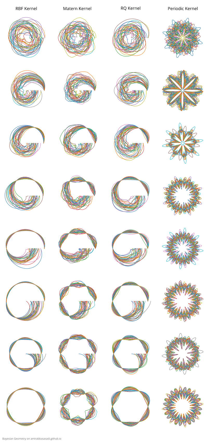
As illustrated above, the posterior shows the update in our belief after inference. I performed the same procedure for 3 other kernels and the posterior after each step is illustrated here:

Defining curves using multiple Gaussian Processes

To model the higher dimensional curves, we can simply use a Gaussian Process for each component along the axis. Furthermore, we assume that processes along the axis are independent. So in the 3D case, we have:

\[t \in [t_a,t_b]\] \[x(t) \sim \mathcal{Gp}(\mathbf{\mu}_x, \mathbf{\Sigma}_x)\] \[y(t) \sim \mathcal{Gp}(\mathbf{\mu}_y, \mathbf{\Sigma}_y)\] \[z(t) \sim \mathcal{Gp}(\mathbf{\mu}_z, \mathbf{\Sigma}_z)\]

If for any reason, you don’t like the assumption of independent components, then you can use a Multi-output Gaussian Process in which the outputs are correlated, If this is the case, see [2] for more details.

Application: Modeling 3D Motion Paths

A potential application of such models is the motion planning problem. Using GP we can address this problem in a probabilistic way so we have a distribution over all possible solutions. If we want to move an object from point $P$ to $Q$ we can express our objective as follows:

\[x(t_a) = P_x, y(t_a) = P_y, z(t_a) = P_z\] \[x(t_b) = Q_x, y(t_b) = Q_y, z(t_b) = Q_z\]

I visualized trajectories sampled from the posterior for 4 different kernels as particles moving from $P$ to $Q$.

Kernel: Squared-Exponential

Kernel: Matern

Kernel: Rational-Quadratic

Kernel: Periodic

Further Reading

We solved the simplest form of the motion planning problem. In real-world problems, we also need to handle possible obstacles in the path. In this case, we can represent the obstacles as constraints over Gaussian Processes, check out [5] to see how to enforce constraints on Gaussian Processes. In this post, I just discussed using Gaussian Process for curves. We can generalize the method to define using other types of manifolds using GP. For instance, see [4] for the application of GP for surface representation.

Also if you are interested in other problems of Stochastic Geometry take a look at [3].

References

• [1] Murphy, K.P., 2012. Machine learning: a probabilistic perspective. MIT press.
• [2] Liu, H., Cai, J. and Ong, Y.S., 2018. Remarks on multi-output Gaussian process regression. Knowledge-Based Systems, 144, pp.102-121.
• [3] Stoyan, D., Kendall, W.S., Chiu, S.N. and Mecke, J., 2013. Stochastic geometry and its applications. John Wiley & Sons.
• [4] Williams, O. and Fitzgibbon, A., 2006, June. Gaussian process implicit surfaces. In Gaussian Processes in Practice.
• [5] Swiler, L.P., Gulian, M., Frankel, A.L., Safta, C. and Jakeman, J.D., 2020. A survey of constrained Gaussian process regression: Approaches and implementation challenges. Journal of Machine Learning for Modeling and Computing, 1(2).